Calorimeter Precision Timing Summer Student projects 2015
*This TWiki contains some introduction and instructions for getting started with summer student projects in the context of the studies for the HGCal calorimeter for HL-LHC.*
Introduction
The projects are summarized in the following sections. The last section summarizes the technical aspects such as software installation, scripting, etc.
Project : Timing impact on e/γ performance
In this project we shall focus on the the impact of timing measurements on the performance for photon/electron reconstruction.
The HGCal readout electronics will provide timing functionality in case the energy (charge) deposited in the Si is sufficientely large (typically > 60fC).
In these cases a time-over-threshold regime will be used to estimate the total charge deposited by means of a Time-to-Digital-Converter (TDC).
The intrinsic jitter of the TDC is expected to be of the order of %$\delta_{t}=50~{\rm ps}$% (Fig. 1) and therefore single cells are expected to have a precision, in the determination of the time-of-arrival,
which is of this order of magnitude. However an electromagnetic object (photon or electron) will produce several hits, depending on its initial energy. Thus,
each e/γ particle will have associated several timing measurements. By making an appropriate choice of the hits with timing information
one can expect the final precision to be %$\sim\delta_{t}/\sqrt{N_{\rm hits}}$% where N<sub>hits</sub> is the total number of hits with timing information.
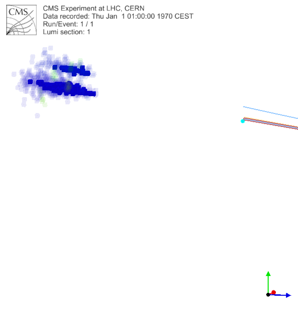
Figure 2 shows an event where two electrons initiate two distinct showers in HGC. Each readout cell is represented by a box which is filled (left hollow)
in case it has timing (has no timing) information associated to it.
| Figure 1 - Jitter in the determination of T<sub>0</sub> for a 100 fC signal. Electronics simulation, credits J. Kaplon. |
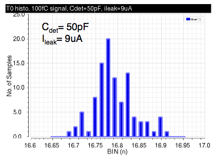 Figure 2 - Event display of a γ→e<sup>+</sup>e<sup>-</sup> event in HGC. Each cell is represented by a square. If filled, the readout cell provides timing information. Credits, L. Gray. |
 We propose that in your project you will study how timing information can be used to:
* identify the origin (vertex) of the reconstructed objects
* remove the superposition of energy deposits from different proton-proton collisions (~140 in the same event at the HL-LHC)
* improve the energy measurement and identification variables used for e/γ
* study the dependency of the performance on the simulation of the behavior of the electronics
The proposed tasks are the following:
* characterise the intrinsic time and spatial resolutions from the hits in a cluster when truth information of the vertex is used
* define a vertex compatibility function (likelihood) by using the time/spatial information of hits associated to a cluster and the reconstructed vertices in the event
* define cleanup or weighting strategy for hits which are likely to come from other vertices in the event
* evaluate the energy resolution for photons before and after the cleanup of pileup is applied
* evaluate how id related variables (e.g. cluster shapes) look like before and after the cleanup of pileup is applied
Once the above is established, and if time allows, alternative simulations where the electronics simulation is varied shall be used to compare the impact on the performance (resolution and identification criteria).
In the next section we describe the technical aspects of how to put this plan into practice!
Software tutorial
The following is meant as a starting point. It describes how to install the software and how to make your first script to analyse and make a plot.
Software installation
To install the software make sure you have already a CERN account and that you asked for some disk space in lxplus (see here
You will need a GitHub
Then login to a lxplus machine (
ssh -Y lxplus.cern.ch) and type the following commands in your work area:cmsrel CMSSW_6_2_0_SLHC25_patch6
cd CMSSW_6_2_0_SLHC25_patch6/src && cmsenv
git cms-merge-topic PFCal-dev:hgc_fasttime_fromtdconset
git clone git://github.com/PFCal-dev/HGCanalysis.git UserCode/HGCanalysis
scram b -j 9
If all was successful,
after you type the last command above,
you should get s.th. like the following in your terminal
...
@@@@ Refreshing Plugins:edmPluginRefresh
>> Pluging of all type refreshed.
>> Done generating edm plugin poisoned information
gmake[1]: Leaving directory `/afs/cern.ch/work/p/psilva/HGCal/Timing/CMSSW_6_2_0_SLHC25_patch6'
Fortunately all this has to be done only once. Next time you login you just have to cd to your directory, then
cd CMSSW_6_2_0_SLHC25_patch6/src
cmsenv
cd UserCode/HGCanalysis
and you'll have all the environment variables set to start working.
We'll be working with the code under the
UserCode/HGCanalysis directory, therefore, in the following, we assume you are in that directory.
Event content
As a starting point we shall use a simple tree
The tree contains the variables described in the table below
Analysing the event content
The best way to analyse the content of the events is by means of a script,
which loads the tree into memory, loops over each event and fills the required histograms.
The script can be written in C or python, whatever you're more comfortable with,
but i'll only show how to do it in python (sorry!).
Below a simple example, meant to get started is given. Create a file called simpleHitAnalysis.py with the following lines: import ROOT
#load library with dictionaries for objects in tree
ROOT.gSystem.Load("libFWCoreFWLite.so")
ROOT.AutoLibraryLoader.enable()
#open ROOT file
fIn=ROOT.TFile.Open('/afs/cern.ch/user/p/psilva/public/hgcsummer2015/HGCROIAnalyzer.root')
#read tree from file
tree=fIn.Get('analysis/HGC')
print 'Preparing to analyse %d events'%tree.GetEntriesFast()
#loop over events in tree
for i in xrange(0,tree.GetEntriesFast()) :
tree.GetEntry(i)
#print event summary
print '-'*50
print '(run,event,lumi)=',tree.run,tree.event,tree.lumi
print '(vx,vy,vz)=',tree.GenVertex.X(),tree.GenVertex.Y(),tree.GenVertex.Z()
print '%d reconstructed vertices' % tree.Vertices.size()
print '%d rec hits, in %d clusters, in %d ROIs' % (tree.RecHits.size(),tree.Clusters.size(),tree.ROIs.size())
save it and run it as:
python simpleHitAnalysis.py
As output you should get something like
Preparing to analyse 2741 events
--------------------------------------------------
(run,event,lumi)= 1 1 1
(vx,vy,vz)= -7.88576362538e-05 -0.000363838364137 -2.62793445587
0 reconstructed vertices
829 rec hits, in 3 clusters, in 2 ROIs
Let's now evolve this example a little bit more to get a starting information of the time of arrival.
Let's compute the average time of arrival from the hits collected in a region of interest.
For that purpose we have to loop over the available RecHits, check which ones belong to which region of interest,
and then average the time of arrival. We shall compare two estimates: a simple average and an energy weighted average.
We can add the following lines to the script you have started above:
# loop over the hits
roiInfo={}
for hit in tree.RecHits:
#select hits with time \
if hit.t_<0 : continue
#get the region of interest
roiId= tree.Clusters[ hit.clustId_ ].roiidx_
#init hit, energy and timing counters
if not roiId in roiInfo : roiInfo[roiId]=[0.,0.,0.,0.]
roiInfo[roiId][0] += 1
roiInfo[roiId][1] += hit.en_
roiInfo[roiId][2] += hit.t_
roiInfo[roiId][3] += hit.t_*hit.en_
#now finish the averages and print information on ROI
for roiId in roiInfo:
#id of the matched particle
particleMatchId=tree.ROIs[roiId].stableid_
#place of interaction of the matched particle (if>317 cm then it happened inHGC)
zinter=ROOT.TMath.Abs(tree.ROIs[roiId].stablez_)
#at least one hit found must be required
if roiInfo[roiId][0]==0 : continue
#finish averages
avgT = roiInfo[roiId][2]/roiInfo[roiId][0]
avgT_weightedE = roiInfo[roiId][3]/roiInfo[roiId][1]
#print information
print 'ROI #%d matched to %d (z_{inter}=%fcm) avgT=%fns avgT_weightedE=%fns' %(roiId,particleMatchId,zinter,avgT,avgT_weightedE)</pre>
This should now print something like
Preparing to analyse 2741 events
--------------------------------------------------
(run,event,lumi)= 1 1 1
(vx,vy,vz)= -7.88576362538e-05 -0.000363838364137 -2.62793445587
0 reconstructed vertices
829 rec hits, in 3 clusters, in 2 ROIs
ROI #0 matched to 22 (z_{inter}=180.653748cm) avgT=0.910208ns avgT_weightedE=0.909215ns
ROI #1 matched to 22 (z_{inter}=169.687393cm) avgT=1.095988ns avgT_weightedE=1.075445ns
In the above example two regions of interest are found in the event, both matched to photons (id=22)
which interact before they hit the calorimeter. This is due to the fact that there is material from the tracker and services
simulated before the calorimeter. The reconstructed average time from the hits produced by the photons is around 1ns,
depending on how the average is computed. We notice also that one photon arrives earlier (0.9ns) than the other (~1.08ns).
At this point one must know how is this RecHit time computed, and why one expects a difference in the time of arrival from two photons coming from the same interaction point.
In figure below we show how the time at which the collision occurs (t<sub>coll</sub>) is related to the observed time
registered in a readout cell (t<sub>obs</sub>) and to the time which is reconstructed, and stored in the event (t<sub>rec hit</sub>):
| Figure 3 - relation between t<sub>coll</sub>, the coordinates of a readout cell and the reconstructed time in the event |
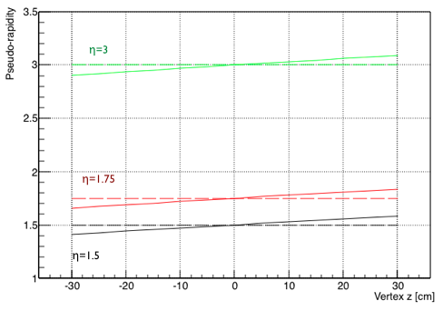
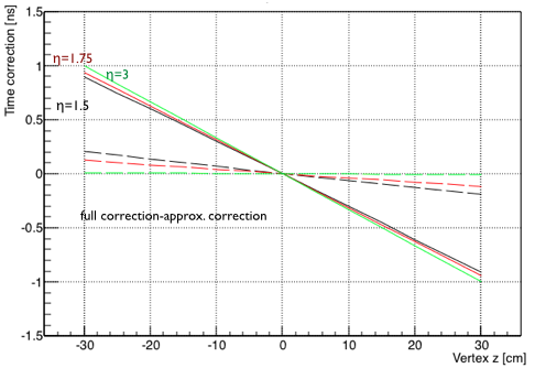
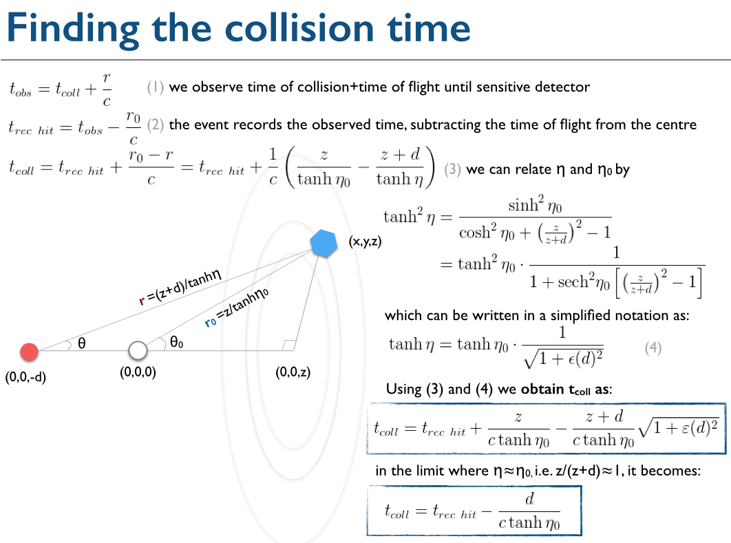 Figure 4 and 5 show the relation between geometrial η and true η as well as the difference in the time corrections required to recover the collision time.
| Figure 4 - relation between geometrical η, (η<sub>0</sub>) i.e. pointing from (0,0,0) to a readout cell is shown in dashed, while the corrected η, i.e. pointing from the vertex of the event to the readout cell is shown as a thick line, as function of the longitudinal position of the vertex
| Figure 5 - Time-correction to apply to the reconstructed hit time as function of the true vertex position. The dashed lines show the difference (in ns) between the full correction and the approximated correction. As expected the difference is diluted for high pseudo-rapidities. |
 Let's now put this in practice by determining t<sub>coll</sub> in the events. For this purpose we shall use an histogram (<a target="_top" href="https://root.cern.ch/root/html/TH1.html">TH1</a> in ROOT).
We add the following lines to the start of the script:
#prepare some control histograms
collTimeH = <a rel="nofollow" href="https://twiki.hep.caltech.edu/twiki/bin/edit/ROOT/TH1F?topicparent=Main.SiTiming;nowysiwyg=0" title="TH1F (this topic does not yet exist; you can create it)">TH1F</a>('colltime_simple',';Collision time [ns];Regions of interest',100,-0.2,0.2)
collTimeFullH = <a rel="nofollow" href="https://twiki.hep.caltech.edu/twiki/bin/edit/ROOT/TH1F?topicparent=Main.SiTiming;nowysiwyg=0" title="TH1F (this topic does not yet exist; you can create it)">TH1F</a>('colltime_full',';Collision time [ns];Regions of interest',100,-0.2,0.2)
This creates two histograms with 100 bins in the range [-0.2,0.2] ns which we will fill.
In the place where the average time estimate is computed add the following lines:
d=tree.GenVertex.z() #true vertex position
z=tree.ROIs[roiId].stablez_ #true interaction in the detector
eta0=tree.ROIs[roiId].eta_ #pseudo-rapidity (geometric)
LIGHTSPEED=29.9792458 #cm/ns
simpleShift = d/(LIGHTSPEED*ROOT.TMath.TanH(eta0))
collTimeH.Fill(avgT+simpleShift-1.0)
epsd2=(ROOT.TMath.Power(z/(z+d),2)-1.0)/ROOT.TMath.Power(<a rel="nofollow" href="https://twiki.hep.caltech.edu/twiki/bin/edit/ROOT.TMath/CosH?topicparent=Main.SiTiming;nowysiwyg=0" title="CosH (this topic does not yet exist; you can create it)">CosH</a>(eta0),2)
fullShift = -(1.0/LIGHTSPEED*ROOT.TMath.TanH(eta0))*(z-(z+d)*ROOT.TMath.Sqrt(1+epsd2))
collTimeFullH.Fill(avgT+fullShift-1.0)
print 'Average time after simple correction %fns full correction %fns' % (avgT+simpleShift-1.0, avgT+fullShift-1.0)
and the following lines to the end of the script, in order to save the histograms to a file.
#save histos to file
fOut=ROOT.TFile.Open('SimpleHitAnalysis.root','RECREATE')
collTimeH.Write()
collTimeFullH.Write()
fOut.Close()
To view the histograms you filled you can open the file in the terminal and do
root -l <a rel="nofollow" href="https://twiki.hep.caltech.edu/twiki/bin/edit/Main/SimpleHitAnalysis?topicparent=Main.SiTiming;nowysiwyg=0" title="SimpleHitAnalysis (this topic does not yet exist; you can create it)">SimpleHitAnalysis</a>.root
TBrowser b
(double click on the file name at the left and then double click on the histogram to display)
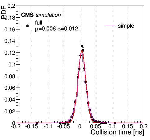
If all went fine you should get plots which are similar to the ones shown below
| Figure 6 - Comparison of the reconstructed collision time from the average time after applying a simple and a full correction. A gaussian fit is superimposed to the results obtained with the full correction. |
 There you go, these are your first plots. You may identify some caveats/shortcuts in what we did to obtain them.
 How exactly were the means computed? Which geometrical information was used in the end? What would happen if a different subset of hits
was used or if individual hits were used instead? etc... the answers to these and other questions are your project :)
In attachment to this twiki you may find a the script which reproduces basically these plots
and which you can use to verify your progress. You can get it from this <a target="_top" href="https://twiki.hep.caltech.edu/twiki/pub/Main/SiTiming/runLocalROIAnalysis.py.txt">link</a>,
and run it as python runLocalROIAnalysis.py -i /afs/cern.ch/user/p/psilva/public/hgcsummer2015/HGCROIAnalyzer.root=
Now you're ready to go! In the next section you'll find a list of samples which you can analyse.
Producing the analysis tree starting from raw CMS events
You can skip this technical note at start. A final technical note: in case you need to produce a ROOT file with the Tree from scratch, i.e. staring from the so called CMS EDM events, all you need is the location of the directory with the original set of simulated events. Then run:
cmsRun test/runHGCROIAnalyzer_cfg.py directory_with_edm_events [output_file_name]
You'll get in your directory a ROOT file with the Tree for analysis.
Location of samples
The table below summarizes where you can find different samples for your analysis.
| Format | Location | Comments |
| Tree | | |
| EDM | =/store/cmst3/group/hgcal/CMSSW/GluGluHtoGG_CMSSW_6_2_0_SLHC25_patch6/HLLHC_Fix/RECO-PU0 | H→γγ (no PU)|
| ^ | /store/cmst3/group/hgcal/CMSSW/VBFHtoInv_CMSSW_6_2_0_SLHC25_patch6/HLLHC_Fix/RECO-PU0 | VBF H→invisible (no PU) |
| ^ | /store/cmst3/group/hgcal/CMSSW/Single22_CMSSW_6_2_0_SLHC25_patch6/RECO-PU0 | γ gun (fixed energy) |
| ^ | /store/cmst3/group/hgcal/CMSSW/Single211_CMSSW_6_2_0_SLHC25_patch6/RECO-PU0 | π<sup>+</sup> gun (fixed energy) |
| I | Attachment | History | Action | Size | Date | Who | Comment |
|---|---|---|---|---|---|---|---|
| |
Electronics.png | r1 | manage | 57.0 K | 2015-06-10 - 11:42 | UnknownUser | |
| |
TimeVision.png | r1 | manage | 77.3 K | 2015-06-10 - 11:42 | UnknownUser | |
| |
coll_time.png | r1 | manage | 204.9 K | 2015-06-10 - 11:42 | UnknownUser | |
| |
coll_time_resol.png | r1 | manage | 28.9 K | 2015-06-10 - 11:42 | UnknownUser | |
| |
eta_correction.png | r1 | manage | 46.4 K | 2015-06-10 - 11:42 | UnknownUser | |
| |
time_correction.png | r1 | manage | 55.9 K | 2015-06-10 - 11:42 | UnknownUser | |
| |
vars.PNG | r1 | manage | 45.4 K | 2015-06-10 - 11:42 | UnknownUser |
Ideas, requests, problems regarding TWiki? Send feedback


